Binary Indexed Tree Binary Indexed Tree (Binary Indexed Tree) #

A Binary Indexed Tree, also named a Fenwick tree after its inventor, was first published by Peter M. Fenwick in 1994 in SOFTWARE PRACTICE AND EXPERIENCE under the title A New Data Structure for Cumulative Frequency Tables. Its original purpose was to solve the problem of calculating cumulative frequencies in data compression, and today it is mostly used to efficiently compute prefix sums and range sums of sequences. For range problems, in addition to the common segment tree solution, you can also consider a Binary Indexed Tree. It can obtain any prefix sum \( \sum_{i=1}^{j}A[i],1<=j<=N \) in O(log n) time, while also supporting dynamic point value modifications (increase or decrease) in O(log n) time. The space complexity is O(n).

Using an array to implement prefix sums makes queries O(1), but for arrays with frequent updates, recomputing prefix sums each time has time complexity O(n). At this point, the advantages of the Binary Indexed Tree become immediately apparent.

I. Concept of a One-Dimensional Binary Indexed Tree #

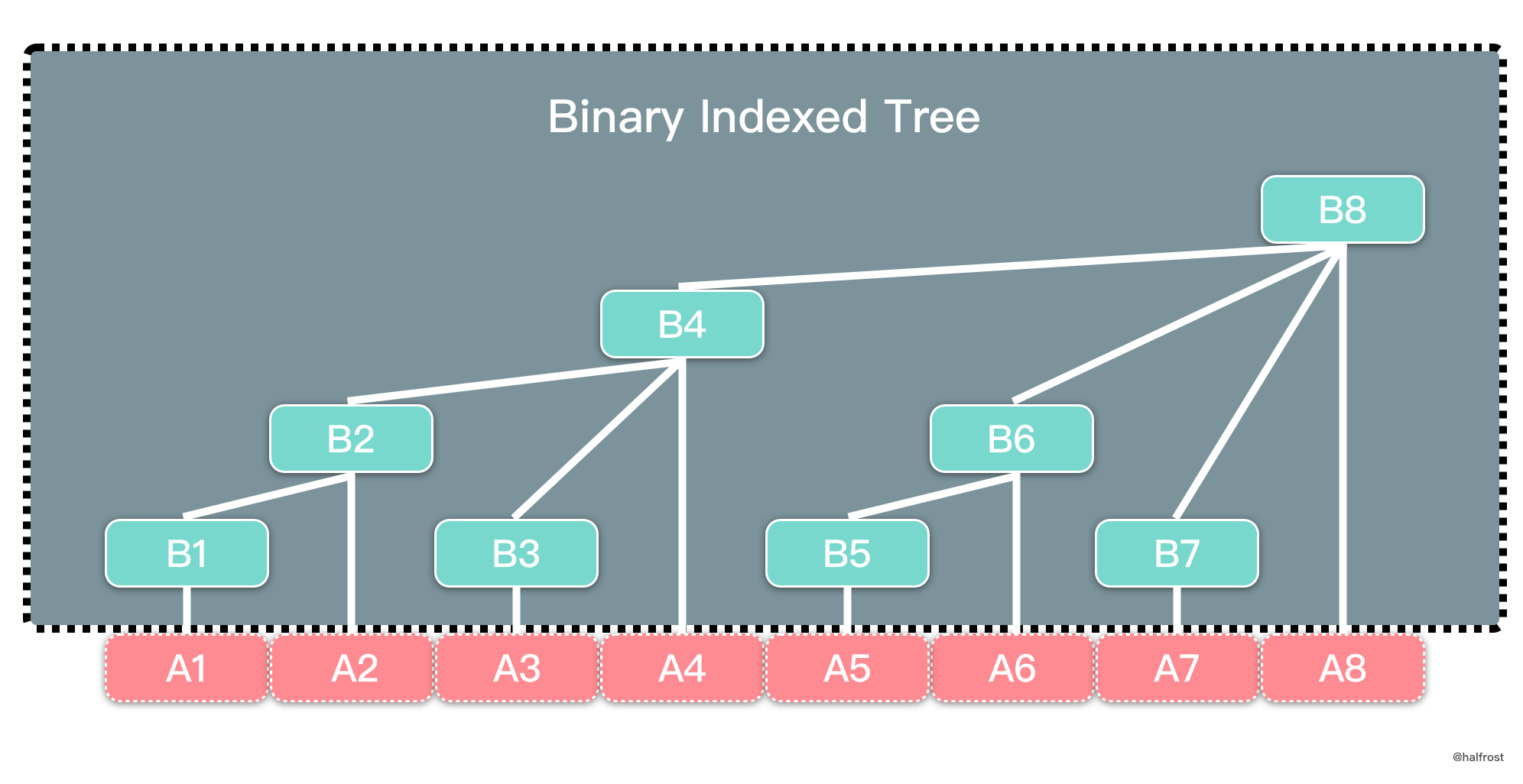
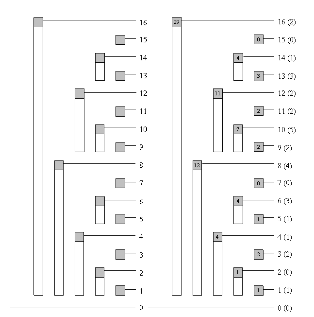
Although the name Binary Indexed Tree contains both “tree” and “array”, its physical form is actually still an array. However, the meaning of each node follows a tree relationship, as shown above. In a Binary Indexed Tree, the parent-child index relationship is \(parent = son + 2^{k}\) , where k is the number of trailing 0s in the binary representation of the child node’s index.

For example, in the figure above, both A and B are arrays. Array A stores data normally, while array B is the Binary Indexed Tree. B4, B6, and B7 are child nodes of B8. The binary representation of 4 is 100, and 4 + \(2^{2}\) = 8, so 8 is the parent node of 4. Similarly, the binary representation of 7 is 111, and 7 + \(2^{0}\) = 8, so 8 is also the parent node of 7.

1. Meaning of Nodes #

In a Binary Indexed Tree, all nodes with odd indices are leaf nodes, representing single points. The value stored in them is the value stored at the same index in the original array. For example, in the figure above, B1, B3, B5, and B7 store the values A1, A3, A5, and A7 respectively. All nodes with even indices are parent nodes. A parent node stores a range sum. For example, B4 stores B1 + B2 + B3 + A4 = A1 + A2 + A3 + A4. The left boundary of this range is the index corresponding to the leftmost leaf node of this parent node, and the right boundary is its own index. For example, the range represented by B8 has left boundary B1 and right boundary B8, so the range sum it represents is A1 + A2 + …… + A8.

By mathematical induction, we can conclude that the index of the left boundary must be \(i - 2^{k} + 1\) , where i is the index of the parent node, and k is the number of trailing 0s in the binary representation of i. Expressing the range sum of even-numbered nodes mathematically:

The code for initializing a Binary Indexed Tree is as follows:

// BinaryIndexedTree define
type BinaryIndexedTree struct {
	tree     []int
	capacity int
}

// Init define
func (bit *BinaryIndexedTree) Init(nums []int) {
	bit.tree, bit.capacity = make([]int, len(nums)+1), len(nums)+1
	for i := 1; i <= len(nums); i++ {
		bit.tree[i] += nums[i-1]
		for j := i - 2; j >= i-lowbit(i); j-- {
			bit.tree[i] += nums[j]
		}
	}
}

The lowbit(i) function returns the value represented by the last 1 at the end after i is converted to binary, namely \(2^{k}\) , where k is the number of trailing 0s in i. We all know that in computer systems, values are represented and stored using two’s complement. The reason is that using two’s complement allows the sign bit and value field to be handled uniformly; at the same time, addition and subtraction can also be handled uniformly. Using two’s complement, lowbit(i) can be calculated in O(1). The two’s complement of a negative number is obtained by inverting every bit of the positive number’s original code and then adding 1. Adding one makes the trailing 0s in the negative number’s two’s complement the same as the trailing 0s in the positive number’s original code. After performing the & operation on these two numbers, the result is lowbit(i):

func lowbit(x int) int {
	return x & -x
}

Readers who still cannot figure it out can look at this example: the binary representation of 34 is \((0010 0010)_{2} \) , and its two’s complement is \((1101 1110)_{2} \) .

The result of lowbit(34) is \(2^{k} = 2^{1} = 2 \)

2. Insertion Operation #

The indices of parent and child nodes in a Binary Indexed Tree satisfy the relationship \(parent = son + 2^{k}\) , so this formula can be used to recurse upward continuously from a leaf node until the maximum node value is reached. There are at most logn ancestor nodes. The insertion operation can implement increasing or decreasing a node value. The code implementation is as follows:

// Add define
func (bit *BinaryIndexedTree) Add(index int, val int) {
	for index <= bit.capacity {
		bit.tree[index] += val
		index += lowbit(index)
	}
}

3. Query Operation #

Query the sum in the interval [1, i] in the Binary Indexed Tree. According to the meaning of the nodes, the following relationship can be derived:

\(B_{i}\) is the value stored in the Binary Indexed Tree. The Query operation is actually a recursive process. lowbit(i) represents \(2^{k}\) , where k is the number of trailing 0s in the binary representation of i. i - lowbit(i) removes the trailing 1 from the binary representation of i. There are at most \(log(i)\) 1s, so the worst-case time complexity of the query operation is O(log n). The implementation code of the query operation is as follows:

// Query define
func (bit *BinaryIndexedTree) Query(index int) int {
	sum := 0
	for index >= 1 {
		sum += bit.tree[index]
		index -= lowbit(index)
	}
	return sum
}

II. Functions of Binary Indexed Trees in Different Scenarios #

Depending on the meaning of the data maintained by nodes, a Binary Indexed Tree can provide different functions to satisfy various range scenarios. Below, we first use the range sum described in the previous example, and then introduce RMQ use cases.

1. Point Increase/Decrease + Range Sum #

This scenario is the most classic scenario for Binary Indexed Trees. Point increase and decrease call add(i,v) and add(i,-v) respectively. For range sum, using the idea of prefix sums, to find the sum of interval [m,n], use query(n) - query(m-1). query(n) represents the sum in interval [1,n], query(m-1) represents the sum in interval [1,m-1], and subtracting the two gives the sum in interval [m,n].

The corresponding LeetCode problems are 307. Range Sum Query - Mutable and 327. Count of Range Sum

2. Range Increase/Decrease + Point Query #

This situation requires a transformation. Define the difference array \(C_{i}\) to represent \(C_{i} = A_{i} - A_{i-1}\) . Then:

Range increase/decrease: increasing every number in interval [m,n] by v only affects the values of 2 single points:

It can be observed that the values of \(C_{m+1}, C_{m+2}, ......, C_{n}\) do not change, and the ones that change are \(C_{m}, C_{n+1}\) . Therefore, in this situation, a range increase only needs to execute add(m,v) and add(n+1,-v).

At this point, point query is finding the prefix sum, \(A_{n} = \sum_{j=1}^{n}C_{j}\) , namely query(n).

3. Range Increase/Decrease + Range Sum #

This situation is an enhanced version of the previous one. The method for range increase/decrease is the same as above: construct the difference array. Here we mainly explain how to perform range queries. First look at how to find the sum of interval [1,n]:

where \(D_{n} = (n - 1) * C_{n}\)

Therefore, to find the range sum, we only need to construct one more \(D_{n}\) .

By analogy, deriving the more general case:

At this point, the range query problem is solved.

4. Point Increase/Decrease + Range Extremum #

The most basic application of a segment tree is range sum, but after replacing the sum operation with the max operation, it can also find the range extremum, and the time complexity does not change at all. What about a Binary Indexed Tree? Can it implement the same function? The answer is yes, but the time complexity will degrade a little.

When a segment tree finds a range sum, it calculates the sums of each small interval and then pushUp successively to update upward. Replacing sum with the max operation has exactly the same meaning: take the maximum value of the small interval, then pushUp successively to obtain the maximum value of the entire interval.

When a Binary Indexed Tree finds a range sum, it updates the influence of the point increase/decrease increment to the fixed interval \([i-2^{k}+1, i]\) . But replacing sum with the max operation changes the meaning. At this point, the increment of a single point has no direct relationship with the interval max value. The brute force method is to compare this point with all values in the interval and take the maximum value, with time complexity O(n * log n). By carefully observing the structure of the Binary Indexed Tree, we can find that it is not necessary to enumerate all intervals. For example, when updating the value of \(A_{i}\) , the affected Binary Indexed Tree indices are \(i-2^{0}, i-2^{1}, i-2^{2}, i-2^{3}, ......, i-2^{k}\) , where \(2^{k} < lowbit(i) \leqslant 2^{k+1}\) . At most k indices need to be updated, and the outer loop is reduced from O(n) to O(log n). The interval itself needs to be compared again each time, requiring O(log n) complexity, so the total time complexity is \((O(log n))^2 \) .

func (bit *BinaryIndexedTree) Add(index int, val int) {
	for index <= bit.capacity {
		bit.tree[index] = val
		for i := 1; i < lowbit(index); i = i << 1 {
			bit.tree[index] = max(bit.tree[index], bit.tree[index-i])
		}
		index += lowbit(index)
	}
}

The point update problem has been solved above. Now look at the range extremum. A segment tree divides intervals evenly, in halves, while a Binary Indexed Tree does not divide evenly. In a Binary Indexed Tree, the interval represented by \(B_{i} \) is \([i-2^{k}+1, i]\) , and “irregular intervals” are divided accordingly. For a Binary Indexed Tree to find the extremum in interval [m,n],

• If \( m < n - 2^{k} \) , then \( query(m,n) = max(query(m,n-2^{k}), B_{n})\)
• If \( m >= n - 2^{k} \) , then \( query(m,n) = max(query(m,n-1), A_{n})\)

func (bit *BinaryIndexedTree) Query(m, n int) int {
	res := 0
	for n >= m {
		res = max(nums[n], res)
		n--
		for ; n-lowbit(n) >= m; n -= lowbit(n) {
			res = max(bit.tree[n], res)
		}
	}
	return res
}

n undergoes at most \((O(log n))^2 \) changes, and finally n < m. The time complexity is \((O(log n))^2 \) .

For this type of problem, here is a classic example problem, 《HDU 1754 I Hate It》:

Problem Description
A habit of comparison is popular in many schools. Teachers really like asking, among students from so-and-so to so-and-so, what is the highest score. This annoys many students. Whether you like it or not, what you need to do now is write a program according to the teacher’s requirements to simulate the teacher’s queries. Of course, the teacher sometimes needs to update the score of a certain student.

Input
This problem contains multiple test cases; please process until the end of file. In the first line of each test case, there are two positive integers N and M ( 0<N<=200000,0<M<5000 ), representing the number of students and the number of operations respectively. Student IDs are numbered from 1 to N. The second line contains N integers, representing the initial scores of these N students, where the i-th number represents the score of the student whose ID is i. Next there are M lines. Each line has one character C (only ‘Q’ or ‘U’) and two positive integers A, B. When C is ‘Q’, it means this is a query operation, asking what the highest score is among students whose IDs are from A to B (including A and B). When C is ‘U’, it means this is an update operation, requiring the score of the student whose ID is A to be changed to B.

Output
For each query operation, output the highest score on one line.

Sample Input
5 6
1 2 3 4 5
Q 1 5
U 3 6
Q 3 4
Q 4 5
U 2 9
Q 1 5


Sample Output
5
6
5
9

After reading the problem, you can quickly realize that it is a point increase/decrease + range maximum problem. Using the idea explained above, write the code:

Since the OJ does not support Go, C code is used here. Here is another Hint: for extremely large input, the performance of scanf() is significantly better than cin.

#include <iostream>
#include <stdio.h>
#include <stdlib.h>
using namespace std;
 
const int MAXN = 3e5;
int a[MAXN], h[MAXN];
int n, m;
 
int lowbit(int x)
{
	return x & (-x);
}
void updata(int x)
{
	int lx, i;
	while (x <= n)
	{
		h[x] = a[x];
		lx = lowbit(x);
		for (i=1; i<lx; i<<=1)
			h[x] = max(h[x], h[x-i]);
		x += lowbit(x);
	}		
}
int query(int x, int y)
{
	int ans = 0;
	while (y >= x)
	{
		ans = max(a[y], ans);
		y --;
		for (; y-lowbit(y) >= x; y -= lowbit(y))
			ans = max(h[y], ans);
	}
	return ans;
}
int main()
{
	int i, j, x, y, ans;
	char c;
	while (scanf("%d%d",&n,&m)!=EOF)
	{
		for (i=1; i<=n; i++)
			h[i] = 0;
		for (i=1; i<=n; i++)
		{
			scanf("%d",&a[i]);
			updata(i);
		}
		for (i=1; i<=m; i++)
		{
			scanf("%c",&c);
			scanf("%c",&c);
			if (c == 'Q')
			{
				scanf("%d%d",&x,&y);
				ans = query(x, y);
				printf("%d\n",ans);
			}
			else if (c == 'U')
			{
				scanf("%d%d",&x,&y);
				a[x] = y;
				updata(x);
			}
		}
	}
	return 0;
}

The above code has been accepted. Interested readers can try this simple ACM problem themselves.

5. Range Overlay + Point Extremum #

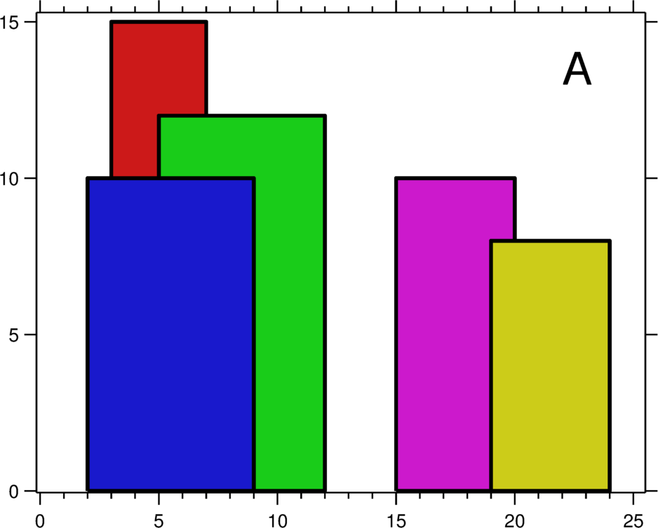
At this point, careful readers may wonder: isn’t this type of problem similar to the second type, “range increase/decrease + point query”? You can consider solving this type of problem using the idea of the second type. However, the troublesome point is that after ranges are overlaid, the update of each point is not directly given as an increase/decrease change; instead, we need to maintain an extremum ourselves. For example, in interval [5,7], the current value is 7, and next a value of 2 is added in interval [1,9]. The correct approach is to add 2 in interval [1,4], add 2 in interval [8,9], and keep interval [5,7] unchanged, because 7 > 2. This is only the case of overlaying 2 intervals. If more intervals are overlaid, more intervals need to be split. At this point, some readers may consider the segment tree solution. Segment trees are indeed powerful tools for solving range overlay problems. Here, the author only discusses the Binary Indexed Tree solution.

Currently LeetCode has 1836 problems, and under the Binary Indexed Tree tag there are only 7 problems. 218. The Skyline Problem can be considered the “hardest” among these 7 BIT problems. This skyline problem belongs to the type of range overlay + point extremum. The author uses this problem as an example to explain common solutions for this type of problem.

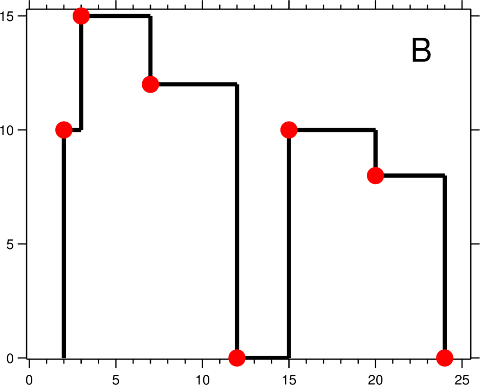
To find the skyline, that is, to find the line along the outer edge of overlapping intervals between buildings, essentially means maintaining the extremum within each interval. There are 2 problems that need to be solved.

1. How to maintain the extremum. When the right boundary of a tall building disappears, among the remaining smaller buildings, the maximum value still needs to be selected as the skyline. There are many remaining overlapping small buildings, and how a Binary Indexed Tree maintains range extrema is the key to solving this type of problem.
2. How to maintain the turning points of the skyline. Some buildings do not completely overlap; partial overlap causes turning points in the skyline. For example, the red turning points marked in the figure above. How does a Binary Indexed Tree maintain these points?

First solve the first problem (maintaining the extremum). A Binary Indexed Tree has only 2 operations, one is Add() and the other is Query(). From the explanation of these 2 operations above, we know that neither operation can satisfy our needs. The Add() operation can be changed to maintain max() within a range. But max() is easy to obtain and hard to “remove”. For example, in the interval [3,7] in the figure above, the maximum value is 15. According to the definition of the Binary Indexed Tree, the extremum in interval [3,12] is still 15. Observing the figure above, we can see that the extremum in interval [5,12] is actually 12. How does a Binary Indexed Tree maintain this kind of extremum? Since the maximum value is hard to “remove”, we need to consider how to make the maximum value “arrive later”. The solution is to change the meaning of the Query() operation from prefix meaning to suffix meaning. Query(i) originally queries the interval [1,i]; now the query interval becomes \([i,+\infty)\) . For example: the extremum in interval [i,j] is \(max_{i...j}\) , and the result of Query(j+1) will not include \(max_{i...j}\) , because the interval it queries is \([j+1,+\infty)\) . After this change, the influence of preceding tall buildings on the accumulated max() extremum of later buildings can be effectively avoided.

The specific approach is to sort the intervals on the x-axis, sorting by x value from small to large. Traverse each interval from left to right. The meaning of the Add() operation is to add the extremum of the suffix interval represented by the right boundary of each interval. In this way, there is no need to consider the problem of “removing” the extremum. Careful readers may have another question: can we traverse intervals from right to left and keep the meaning of Query() as the prefix interval? This is feasible and can solve the first problem (maintaining the extremum). But this processing method will run into trouble when solving the second problem (maintaining turning points).

Now solve the second problem (maintaining turning points). If Query() with prefix meaning is used, at a single point i, in addition to considering intervals ending at this point, it is also necessary to consider intervals starting at this single point i. If Query() has suffix meaning, there is no such problem. The interval \([i+1,+\infty)\) does not need to consider intervals ending at single point i. The Binary Indexed Tree implementation for this problem is as follows:

const LEFTSIDE = 1
const RIGHTSIDE = 2

type Point struct {
	xAxis int
	side  int
	index int
}

func getSkyline3(buildings [][]int) [][]int {
	res := [][]int{}
	if len(buildings) == 0 {
		return res
	}
	allPoints, bit := make([]Point, 0), BinaryIndexedTree{}
	// [x-axis (value), [1 (left) | 2 (right)], index (building number)]
	for i, b := range buildings {
		allPoints = append(allPoints, Point{xAxis: b[0], side: LEFTSIDE, index: i})
		allPoints = append(allPoints, Point{xAxis: b[1], side: RIGHTSIDE, index: i})
	}
	sort.Slice(allPoints, func(i, j int) bool {
		if allPoints[i].xAxis == allPoints[j].xAxis {
			return allPoints[i].side < allPoints[j].side
		}
		return allPoints[i].xAxis < allPoints[j].xAxis
	})
	bit.Init(len(allPoints))
	kth := make(map[Point]int)
	for i := 0; i < len(allPoints); i++ {
		kth[allPoints[i]] = i
	}
	for i := 0; i < len(allPoints); i++ {
		pt := allPoints[i]
		if pt.side == LEFTSIDE {
			bit.Add(kth[Point{xAxis: buildings[pt.index][1], side: RIGHTSIDE, index: pt.index}], buildings[pt.index][2])
		}
		currHeight := bit.Query(kth[pt] + 1)
		if len(res) == 0 || res[len(res)-1][1] != currHeight {
			if len(res) > 0 && res[len(res)-1][0] == pt.xAxis {
				res[len(res)-1][1] = currHeight
			} else {
				res = append(res, []int{pt.xAxis, currHeight})
			}
		}
	}
	return res
}

type BinaryIndexedTree struct {
	tree     []int
	capacity int
}

// Init define
func (bit *BinaryIndexedTree) Init(capacity int) {
	bit.tree, bit.capacity = make([]int, capacity+1), capacity
}

// Add define
func (bit *BinaryIndexedTree) Add(index int, val int) {
	for ; index > 0; index -= index & -index {
		bit.tree[index] = max(bit.tree[index], val)
	}
}

// Query define
func (bit *BinaryIndexedTree) Query(index int) int {
	sum := 0
	for ; index <= bit.capacity; index += index & -index {
		sum = max(sum, bit.tree[index])
	}
	return sum
}

This problem can also be solved using a segment tree and sweep line. Solving this problem with a sweep line and Binary Indexed Tree is very fast. The segment tree is slightly slower.

III. Common Applications #

This chapter discusses common applications of Binary Indexed Trees.

1. Finding Inversion Pairs #

Given a permutation P of \( n \) numbers \( A[n] \in [1,n] \) , find the number of pairs \( (i,j) \) satisfying \(i < j \) and \( A[i] > A[j] \) .

This problem is the classic inversion count problem. If a naive algorithm is used, it enumerates i and j and determines the values of A[i] and A[j] for counting. If A[i] > A[j], the counter is incremented by one. After the statistics are complete, the value of the counter is the answer. The time complexity is \( O(n^{2}) \) , which is too high. Is there an \( O(log n) \) solution?

If the problem changes to \( A[n] \in [1,10^{10}] \) , the solution idea remains the same, except that one more step, discretization, is added at the beginning.

Assume the first step requires discretization. First convert the numbers in the sequence into integers from 1 to n in sorted order. Assign duplicate data the same number, and assign continuous numbers to missing data. This maps the original sequence into an array B of 1,2,…,n. Note that the elements stored in array B are also unordered and are mapped from the original array. For example, the original array is int[9,8,5,4,6,2,3,8,7,0]. The number 8 is repeated in the array, and the number 1 is missing. Mapping this array into the interval [1,9], the adjusted array B is int[9,8,5,4,6,2,3,8,7,1].

Then create a Binary Indexed Tree to record the prefix sum of such an array C (indices starting from 1): if the number i in this permutation [1, N] has currently appeared, then the value of C[i] is 1; otherwise it is 0. Initially, all values in array C are 0. Start traversing from the first element of array B, and perform the operation on the Binary Indexed Tree of adding 1 to the B[j]-th value of array C. Then query in the Binary Indexed Tree how many numbers are less than or equal to the current number B[j] (that is, use the Binary Indexed Tree to query the prefix sum of interval [1,B[j]] in array C). The current total number inserted i minus the total number of elements less than or equal to B[j] gives the number of elements greater than B[j], which is added to the counter.

func reversePairs(nums []int) int {
	if len(nums) <= 1 {
		return 0
	}
	arr, newPermutation, bit, res := make([]Element, len(nums)), make([]int, len(nums)), template.BinaryIndexedTree{}, 0
	for i := 0; i < len(nums); i++ {
		arr[i].data = nums[i]
		arr[i].pos = i
	}
	sort.Slice(arr, func(i, j int) bool {
		if arr[i].data == arr[j].data {
			if arr[i].pos < arr[j].pos {
				return true
			} else {
				return false
			}
		}
		return arr[i].data < arr[j].data
	})
	id := 1
	newPermutation[arr[0].pos] = 1
	for i := 1; i < len(arr); i++ {
		if arr[i].data == arr[i-1].data {
			newPermutation[arr[i].pos] = id
		} else {
			id++
			newPermutation[arr[i].pos] = id
		}
	}
	bit.Init(id)
	for i := 0; i < len(newPermutation); i++ {
		bit.Add(newPermutation[i], 1)
		res += (i + 1) - bit.Query(newPermutation[i])
	}
	return res
}

The newPermutation in the above code is the mapped and adjusted array B. Traverse array B and insert elements into the Binary Indexed Tree in order. For example, array B is int[9,8,5,4,6,2,3,8,7,1]. Now inserting 6 into the Binary Indexed Tree means that the element 6 has appeared. query() queries whether elements have appeared in interval [1,6], and the interval prefix sum represents the total number of occurrences of elements in the interval. If k elements have appeared and 5 elements have currently been inserted, then the difference 5-k is the number of inverted elements, and these elements must be greater than 6. This method constructs the Binary Indexed Tree in forward order.

Another method is to construct the Binary Indexed Tree in reverse order. For example, the following code:

	for i := len(s) - 1; i > 0; i-- {
		bit.Add(newPermutation[i], 1)
		res += bit.Query(newPermutation[i] - 1)
	}

Because insertion is performed in reverse order, before each Query, the indices of the elements must be greater than the current i. Elements with indices greater than i and values smaller than A[i] can form inversion pairs with i. Query finds the total number of elements in interval [1, B[j]], which is the total number of inversion pairs.

Note that when calculating inversion pairs, do not count duplicates. For example, if you calculate the numbers before index j whose values are greater than B[j], and also count the numbers after index j whose values are less than B[j], this produces many duplicates. Because an index k before index j will also look for numbers after index k whose values are less than B[k], causing repeated counting. Therefore, either uniformly find elements with smaller indices but larger values, or uniformly find elements with larger indices but smaller values. Do not calculate in a mixed way.

The corresponding LeetCode problems are 315. Count of Smaller Numbers After Self, 493. Reverse Pairs, and 1649. Create Sorted Array through Instructions

2. Finding Range Inversion Pairs #

Given a sequence \( A[n] \in [1,2^{31}-1] \) of \( n \) numbers, then given \( n \in [1,10^{5}] \) queries \( [L,R] \) , each query asks for the number of index pairs \( (i,j) \) in interval \( [L,R] \) satisfying \( L \leqslant i < j \leqslant R \) and \( A[i] > A[j] \) .

This problem has one more range constraint than the previous problem. This range constraint affects the selection of inversion pairs. For example: [1,3,5,2,1,1,8,9,8,6,5,3,7,7,2], find the inversion count in interval [3,7]. The element 2 is within the interval, and there are only 2 elements greater than 2. Elements 3 and 5 are outside the interval, so 3 and 5 cannot participate in inversion counting. There are also only 2 elements smaller than 2. The 3 yellow-marked 1s are all smaller than 2, but the first 1 cannot be counted because it is outside the interval.

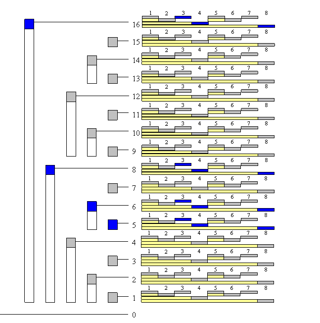
First sort all query intervals by nondecreasing right endpoint, as shown in the figure below.

Here, the query intervals can also be sorted by nonincreasing left endpoint. If sorted this way, the Binary Indexed Tree below needs to be constructed by inserting in reverse order, and what is found are inversion pairs with later indices but smaller element values. Both methods can be implemented; here, one of them is chosen for explanation.

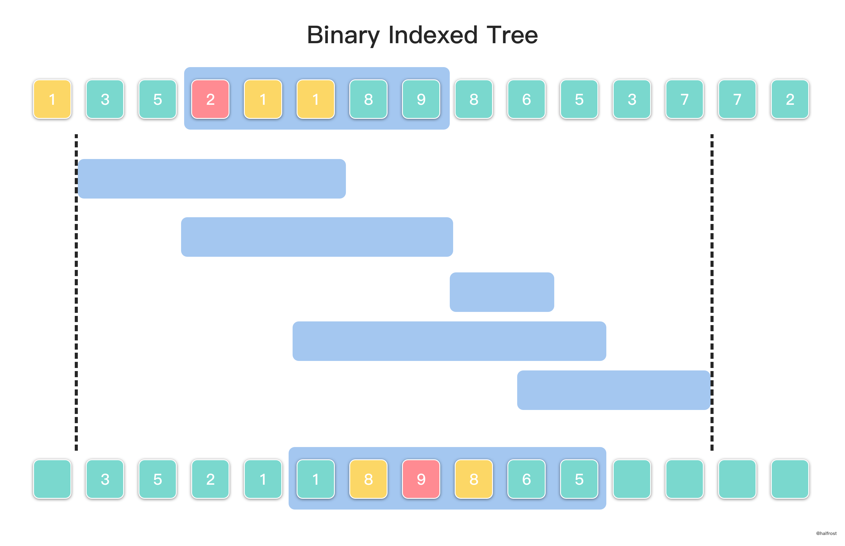
The range covered by the overall intervals determines the range of numbers to be inserted into the Binary Indexed Tree. As shown above, the overall interval is located in [1,12], so elements with indices 0, 13, and 14 do not need to be considered. They will not be used, so they also do not need to be inserted into the Binary Indexed Tree.

In the process of finding range inversion pairs, an auxiliary array C[k] is also needed. The meaning of this array is: for the element with index k, before it is inserted into the Binary Indexed Tree, how many elements have values smaller than A[k]. For example, the element value at index 7 is 9. C[7] = 6, because the elements currently smaller than 9 are 3, 5, 2, 1, 1, and 8. The meaning of this auxiliary array C[k] is to find the number of elements with indices smaller than it and element values also smaller than it.

Since the intervals are sorted by right endpoint here, the Binary Indexed Tree is constructed by inserting in forward order. This way, interval queries from left to right can obtain results successively. As shown in the bottom row of the figure above, suppose the current query has reached the 4th interval. The 4th interval contains element values 1,8,9,8,6,5. Currently, the Binary Indexed Tree is being constructed by inserting from left to right, and element values with indices in interval [1,10] have already been inserted, namely the inserted values shown in the figure. Now traverse all elements in the query interval. Query(A[i] - 1) - C[i] is the total number of inversion pairs for index i in the current query interval. For example, element 9:

Inserting element A[i] to construct the Binary Indexed Tree comes first. Query() queries the current global situation, namely querying the total number of all elements smaller than element 9 in the index interval [1,10]. It is not hard to see that all elements are smaller than element 9, so the result obtained by Query(A[i] - 1) is 9. C[7] is the total number of elements smaller than element 9 before element 9 was inserted into the Binary Indexed Tree, which is 6. Subtracting the two gives the final result 9 - 6 = 3. Looking at the figure above, it is also easy to see that the result is correct: within the interval, there are only 3 elements with indices greater than 9’s index and element values smaller than 9, corresponding to indices 8, 9, and 10, with element values 8, 6, and 5 respectively.

Summary:

1. Discretize array A[i]
2. Sort all intervals by nondecreasing right endpoint
3. According to the sorted intervals, traverse each interval from left to right. Based on the range of elements covered by intervals from left to right, insert A[i] into the Binary Indexed Tree from left to right, and calculate the auxiliary array C[i] before inserting each element.
4. Traverse all elements in each interval in order. For each element, calculate Query(A[i] - 1) - C[i]. Accumulating the results of inversion pairs gives the total number of all inversion pairs in this interval.

3. Finding Inversion Pairs on a Tree #

Given a tree with \( n \in [0,10^{5}] \) nodes, find for each node the number of nodes in its subtree whose node numbers are smaller than it.

The problem of inversion pairs on a tree can be converted into an array through preorder traversal of the tree. Let a certain node on the tree be i, the order visited by preorder traversal be pre[i], and the number of child nodes of i be a[i]. Then after conversion into an array, the interval managed by i is [pre[i], pre[i] + a[i] - 1], and the problem can then be converted into a range inversion pair problem for solving.

IV. Two-Dimensional Binary Indexed Tree #

A Binary Indexed Tree can be extended to two dimensions, three dimensions, or higher dimensions. A two-dimensional Binary Indexed Tree can solve statistical problems on a discrete plane.

// BinaryIndexedTree2D define
type BinaryIndexedTree2D struct {
	tree [][]int
	row  int
	col  int
}

// Add define
func (bit2 *BinaryIndexedTree2D) Add(i, j int, val int) {
	for i <= bit2.row {
		k := j
		for k <= bit2.col {
			bit2.tree[i][k] += val
			k += lowbit(k)
		}
		i += lowbit(i)
	}
}

// Query define
func (bit2 *BinaryIndexedTree2D) Query(i, j int) int {
	sum := 0
	for i >= 1 {
		k := j
		for k >= 1 {
			sum += bit2.tree[i][k]
			k -= lowbit(k)
		}
		i -= lowbit(i)
	}
	return sum
}

If what a one-dimensional Binary Indexed Tree maintains is a statistical problem on the number line,

then what a two-dimensional array maintains is a statistical problem in a two-dimensional coordinate system. X and Y both respectively satisfy the properties of a one-dimensional Binary Indexed Tree.